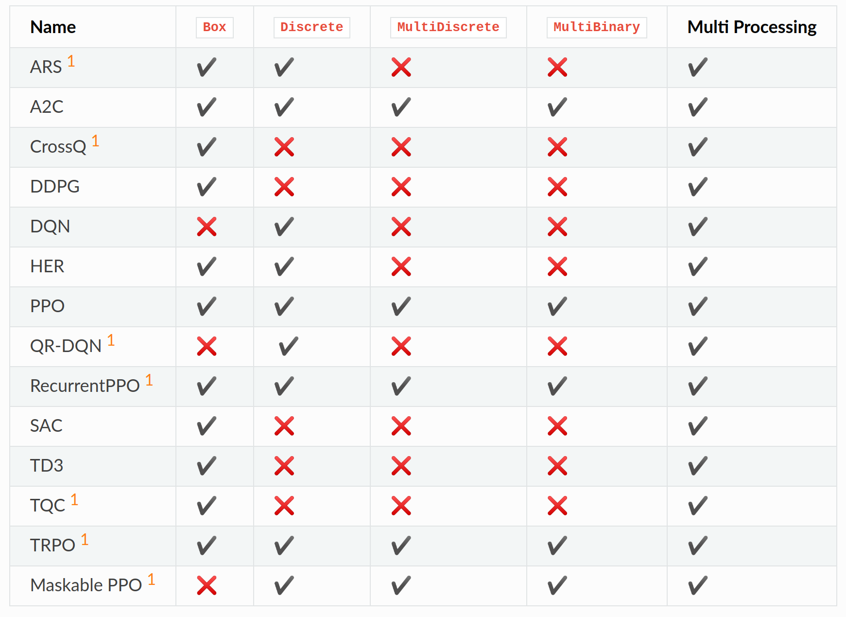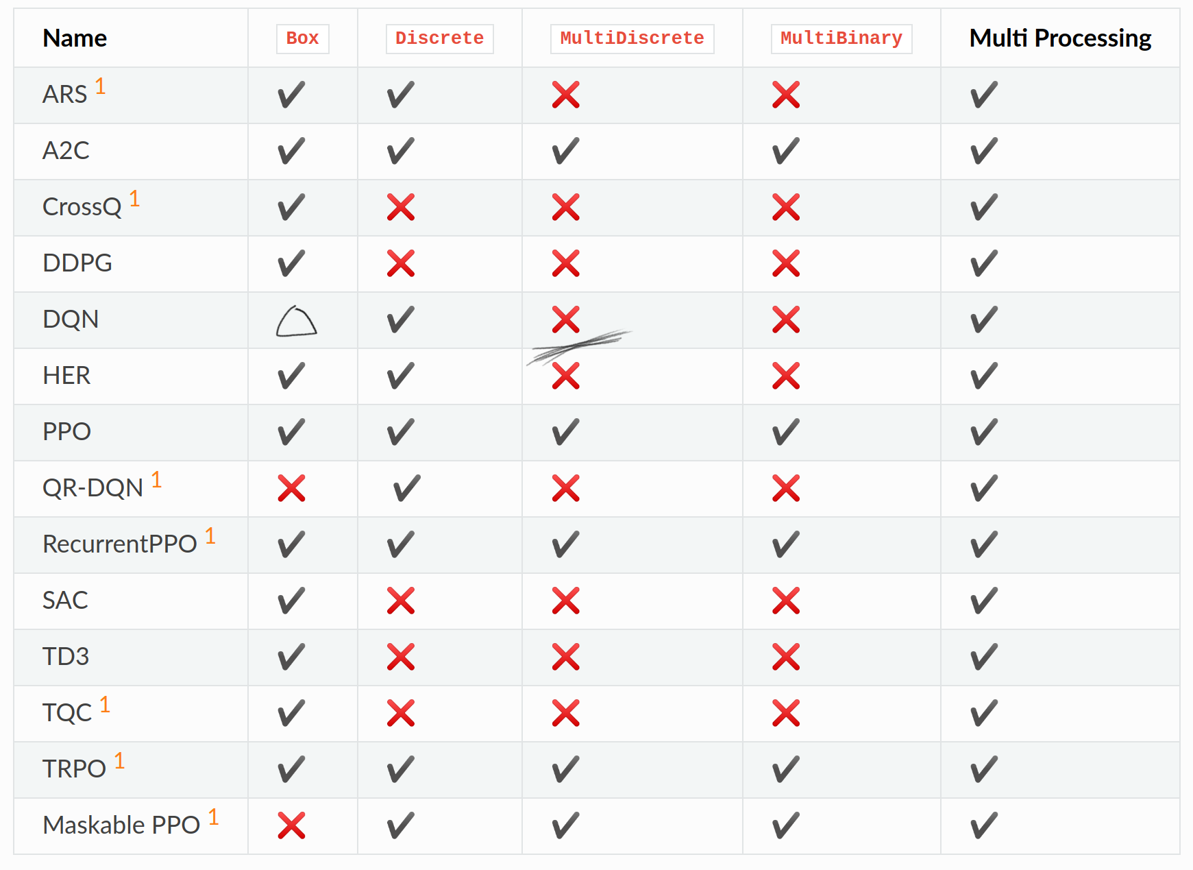
DQN is still missing support for MultiDiscrete action spaces. That’s the other major limitation I want to address. It also says MultiBinary is missing, but that’s just a weird MultiDiscrete so I’ll ignore it.
Box is also only half solved, but the full Box action space isn’t just about continuous action, it’s also an action space for multiple actions.
Actions with multiple decisions
MultiDiscrete actions represent situations where you need to make multiple independent decisions simultaneously in each step.
Think about controlling a character in a game where you need to be doing multiple things at once, you might need to decide movement direction, where to aim, or whether to use special abilities at any given moment. For each of these, you might have different buttons for controling them.
Let me use an example. The agent has an Xbox controller as the action space. At any timestep, the agent needs to decide to press:
- Face buttons: Press A, B, X, Y or not (4 binary decisions)
- Joysticks: Left stick direction, right stick direction (two 2D continuous inputs)
- Triggers/Bumpers: Left trigger, right trigger, left bumper, right bumper (4 more binary decisions, or 2 binary and 2 continuous actions)
I’ll call these individual decisions a subaction. The complete action for that timestep is the combination of all subaction choices. In general, subactions are unordered set, they are executed simultaneously.
In this post, I’ll be going over how to handle composite actions.
The standard approach
The easiest way, and how many tutorial for Q-learning does is by making it a single action space by representing it as a cartesian product, or using a hand selected subset of it. This means, for every additional possible action, the possible actions that the agent needs to consider each step grows exponentially.
For the controller case, it would be
- Face buttons: \(2^4 = 16\) combinations
- Joysticks: \(8^2 = 64\) combinations (if discretized to 8 directions each)
- Triggers/bumpers: \(2^4 = 16\) combinations
For a total of \(16 \times 64 \times 16 =16,384\) possible actions. If you want to consider joystick and trigger to have variable strengths instead of being discretized, this would grow even more.
The size of the action space isn’t the only problem here, the biggest problem is that every action is treated completely differently from each other. To the agent, an action with one different component would be represented as differently as a completely different different action. This would make training take so much longer, because associating actions would be needlessly hard.
It would be much better to keep subactions separate, sample them individually, and combine them into the final action. That way, it would reduce the represented actions, and also relate similar actions together better. This is how every other RL algorithm does it anyway.
How to make sampling subactions easier
Q-values represent expected future reward for taking a particular action. But what should Q-values mean for multiple simultaneous actions?
Q-values only make sense for a complete action that you’ve decided to take, which is why the standard approach has a full table of every combination. We can make sampling much easier if each subaction had its own function to sample, which has predictable effects in the overall Q-value. How could we do this? The simplest way might be to have functions for each subactions, and let the Q-value be the sum of them:
\[Q(\mathbf{a}; s) = \displaystyle\sum_{i = 1}^n Q(a_i; s)\]I tried this initially and it kind of worked, but there’s an identifiability problem during training: Even if you’ve identified \(Q(\mathbf{a}; s)\) for every possible $\mathbf{a}$ in a given state, you still can’t uniquely reconstruct each \(Q(a_i; s)\). If one subaction’s Q-values have a constant added while another’s have the same constant subtracted, the sum remains unchanged. This is a problem for trying to figure out gradients, because there wouldn’t be a unique minimum, there will be entire symmetry group with the same minimum loss, where some of the minima have worse training dynamic.
But this the exact same problem that Dueling Networks faced, which means we can use the same trick as it!
They solved this by adding a state value that is independent of actions, and replacing action values with action advantages where the average over possible actions is subtracted. We can apply the same fix: add an action-independent state value, and replace all subaction values with subaction advantage.
\[Q(\mathbf{a}; s) = V(s) + \displaystyle\sum_{i = 1}^n \left ( Q(a_i; s ) - \displaystyle\sum_{a'_i \in A_i} \frac{1}{|A_i|} Q(a'_i; s) \right)\]This approach works well, and it’s essentially what the Action Branching Architectures paper implements. They create independent advantages for each subaction and add them to a state value to make the Q-value.
\[\]The Independence Problem
While the Action Branching paper treats independent subaction sampling as a feature, I think it’s actually a limitation.
Consider an agent learning to use an art program. For each brush stroke, it needs to simultaneously decide:
- What to draw: Sun, tree, lake, or cloud
- Where to place it: Top, middle, bottom of canvas
- Which color: Yellow, green, blue, or white
You could draw a sun on the top in yellow, a lake in the middle in blue, and those combinations would make sense.
But with independent sampling, each subaction would have no idea on what it already chose, so you might get “draw sun + use blue + place at bottom” resulting in a blue sun underwater, or “draw lake + use yellow + place at top” giving you a floating yellow lake in the sky!
In Action Branching, the authors argue that the shared state representation can coordinate decisions. The idea is that the state embedding would have already decided which action it should take, and the independent subactions will all agree to take the action according to the decision.
But it’s not obvious how this could work. Unlike policy gradient methods where you only make one per subaction, in DQN you construct a Q-function that is defined over all possible actions. If the subaction advantage values are generated independently, the resulting Q-function necessarily has no correlation between different subactions for a given environment state.
Autoregressive Action Sampling
To handle actions being dependent on each other while keeping the sampling easy, I propose an autoregressive action sampling method, where each subaction are conditioned on previously sampled subactions within the same step.
To explain this, let me use the currying interpretation that helped last time. The Q-value function \(Q(s, A)\) could be written as \(Q(s)(a_0)(a_1)...(a_n)\) for some order of subactions. The idea is to sample one action at a time to build up the final Q-value, but we need to be careful a bit because this is actually doing two steps at a time.
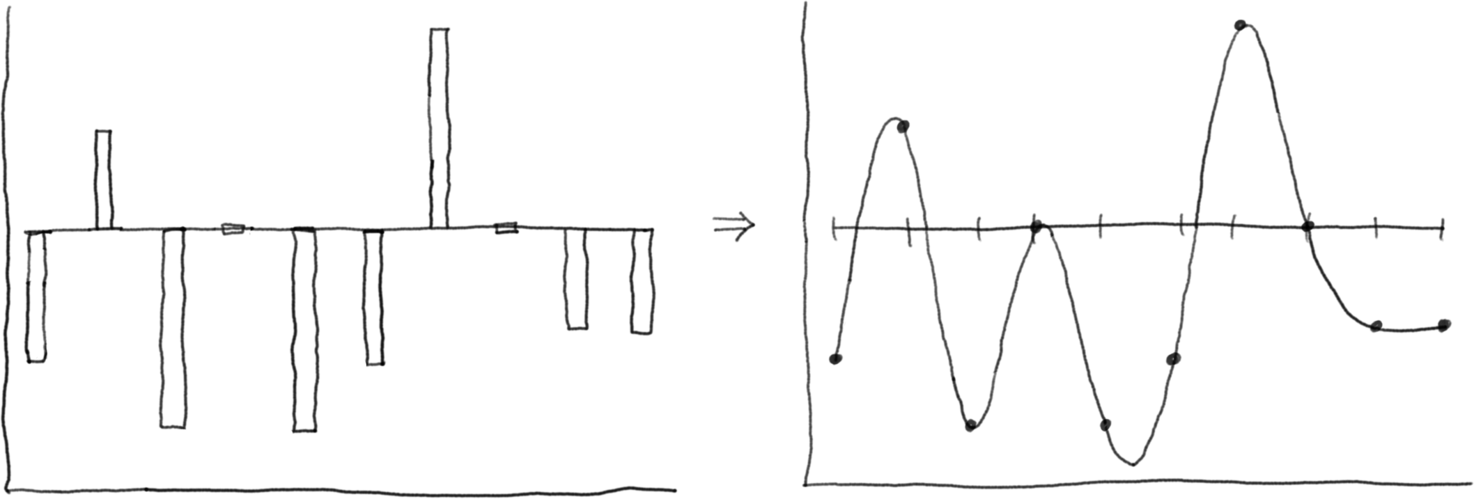
When I write \(Q(s)\) or \(Q(s)(a_0)...(a_k)\), the result is a function. What we want is for each step to also be producing a value, so that each subaction can be sampled. I want a Q-advantage function \(F\) that can turn any of these intermediates and produce the advantage function for the next specific subaction. For discrete actions, this looks like a table while for continuous actions, this looks like a spline curve.
So using these, the steps to sample the full action for a step is to
- Make embedding \(Q(s)\) and state value that does not depend on the action for this step
- Make \(F(Q(s))\) that is a function of the first subaction, and sample \(a_0\)
- Make the next embedding \(Q(s)(a_0)\) from sampled subaction
- sample from \(F(Q(s)(a_0))\) to get \(a_1\), and repeat from 3 until finished
Then the Q-value for the state is the sum of state value and the subaction advantages.

This way, each subaction decision can account for what was already decided. In the earlier drawing example, if it decided to draw a tree as the first subaction, it could then decide to start from the trunk, and then choose brown as the color.
Model Architecture
Autoregressive action sampling needs to do two things, sample actions and evaluate a value given the state and action taken. Sampling autoregressively is a bit slow, since before being able to sample a new action, all the action before it needs to be sampled first. Evaluation in other hand can be faster, since you already have all of the action that needs to be taken, so the overhead of sampling individually is not there.
For a recurrent network, these two will be done exactly the same way. But transformers can take advantage of faster evaluation. Transformers can also use optimizations for sampling like KV caching for each sampling step, or architectures like Grouped Query Attention and Multi Latent Attention.
At first I’ve tried using a full self attention with the state and action embedding concatenated together, but this seems to perform worse than Action Branching. I’ve spent a lot of time trying to figure out why, but it seems there needed to be a clear separation between the states and action. Cross Attention works much better, with the states being the query and action being the key and value. At the worst of cases, it would behave like Action Branching.
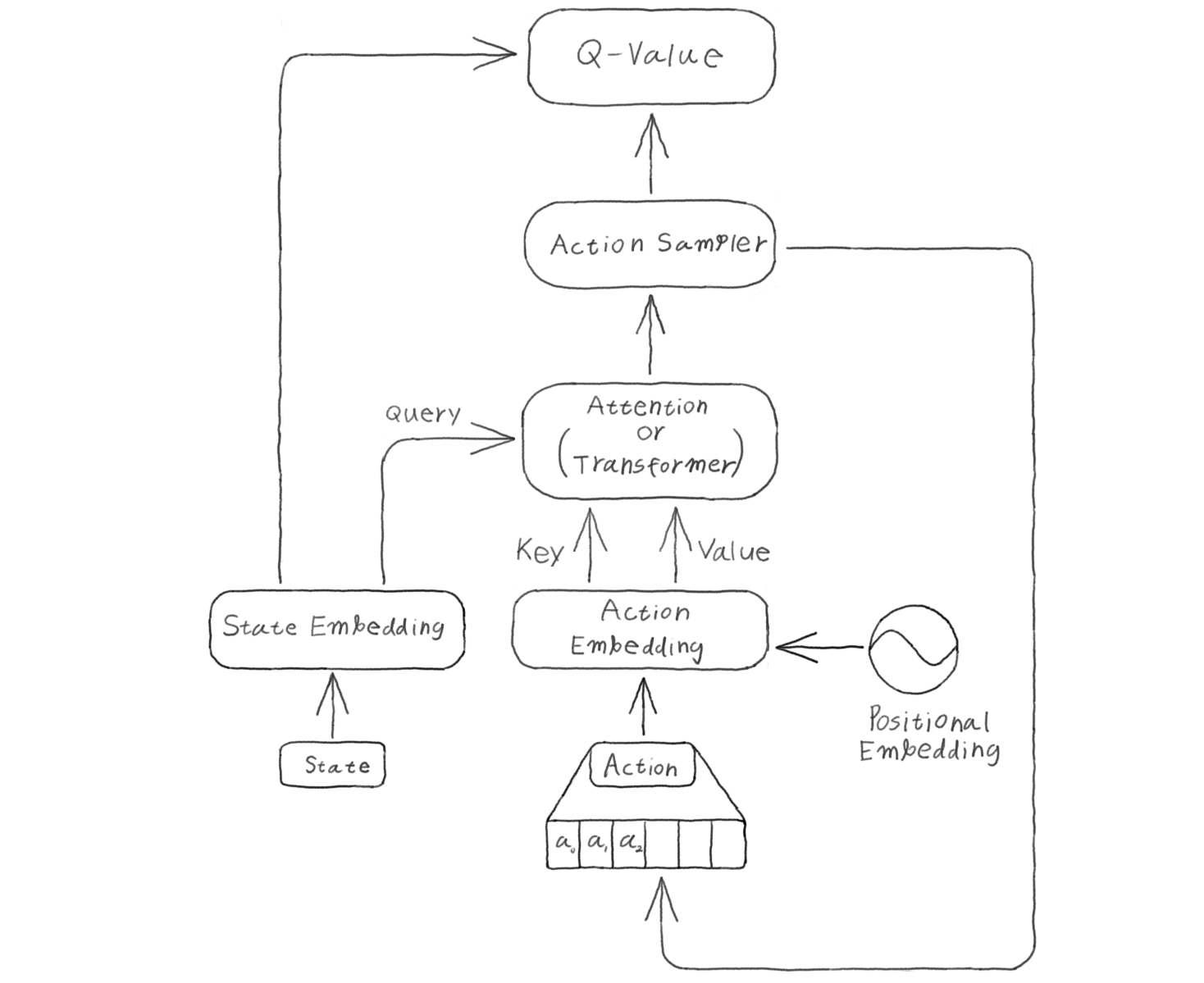
What I like to do is to add a beginning of sequence tokens before the first action token, so that there are something for the state embedding to attend to for the first sampling.
Subaction Ordering Problem
With an autoregressive sampling, there needs to be an order to sample the subactions, but how would you decide the order?
In general, subactions are a set with no order. At the same time, there might be a more natural order to decide, but it’s impossible to know without some domain knowledge which order is better or not. You need to already know something about the environment.
Picking a predetermined action order at random is what I’m doing right now and this works, but feels unsatisfying. I have two ideas on how to make this better, but I haven’t been able to make them work yet. They are at the Action Order section
Conclusion
I couldn’t really get a clear result after many trial and error, and I underestimated just how well the prior work, Action Branching works well in practice. I can come up with cases where Action Branching would definitely fail, but I don’t have any environments where that might be a problem yet.
Q-learning can be used to handle actions which have multiple subactions to them just fine, without hitting the combinatorial explosion problem that people typically face. I’ve shown that combined with the spline action space for continuous action, Q-learning can be used for any environments just like policy gradient methods.
Addendum
Prior Works
The core idea of handling multiple subactions with Q-learning was introduced in Action Branching Architectures for Deep Reinforcement Learning. They use independent Q-functions for each subaction and combine them using the dueling network architecture.
I had a similar idea independently, but found their paper while researching for this blog and realized they had already solved the basic version of this problem. Their approach works well for many cases, but struggles with scenarios that require coordinated subaction strategies.
The autoregressive approach I’m proposing builds on their foundation but adds the ability to handle action dependencies through sequential conditioning.
Action Order
Dynamic Action Order
If I could try different orderings and learn which order performs better dynamically, that could be better than deciding a random order.
To make dynamic action order to work, I imagined sampling a permutation matrix that determines the action sampling order, and learn orders that generally improve rewards as the model trains. This would need some algorithm to figure out what order should be used.
To figure out an algorithm, I made a few assumptions. If one subaction order is better than another order, then the better order would have less uncertain prediction, and the temporal difference loss could be used as a proxy for uncertainty.
To simplify, I’ll also assume that TD loss scale is determined only by the order of subactions and is the sum of pairwise values associated with consecutive subactions in that order.
We can’t just compare the TD loss per subaction, for the same reason that TD loss needed to be summed over the state value and action value. A subaction sampled earlier might make another subaction sampled later to have better options.
Given these assumption, I could formulate this as an optimization problem:
- $n$ vertices are connected by directed edges with unknown weights. Given samples of hamiltonian path with the sum of edge weights, what is the best path that likely minimizes the total weight from the given information gathered from sampling?
Each vertices represent a subaction, and the directed edge between them are the order of sampling, and the weights are how much they contribute to the total TD loss.
This is just a traveling salesman problem, if the edge weights are known. You could maybe setup a linear equation to figure out the weights as you sample, but that would make a $n^2$ by $n^2$ matrix that needs to be solved, which would already be $O(n^6)$ even before the TSP step.
Maybe there is a better way to figure out the weights, or maybe there is a way that doesn’t even need to figure out the weight? I got stuck trying to figure this out.
The assumption that TD loss scale is only determined by order pairs doesn’t really hold up probably, reward scale already matters on which action was taken first regardless of how far ago it was sampled.
So, I could try another assumption. Instead of only consecutive subaction having interaction, suppose that every pair of subaction has an ordering preference, where the values are assigned on whether a subaction is before another, regardless of how far apart they are. The TD loss would be the sum of all ordering preference.
This would change the problem into a Linear Ordering Problem if the values are known, which is also a known NP-hard problem.
I couldn’t figure out a good way to do this, and this is about the time I started thinking about Action Latents so I’ve put it on indefinite hold.
Latent Action Space
This is the other idea that I came up while writing this blog post, and I’m still exploring.
If picking an order is a problem because I don’t know which order would be better, what if I make my own representation of actions, and sample from that?
Imagine you’re riding a bicycle. You don’t consciously think of what muscles to pull at what moment, you have a conceptual understanding of what to do, and let your muscle memory figure out the small movements. In order for your body to figure that out, it takes a while of trying.
Latent action space is kind of like that, instead of dealing with the raw actions, it could learn how to conceptualize actions in meaningful ways, and act on that space instead.
The learned representation would be sampled in an order, but the representation could be learned in a way that the order it gets sampled would be the optimal order to be sampled.
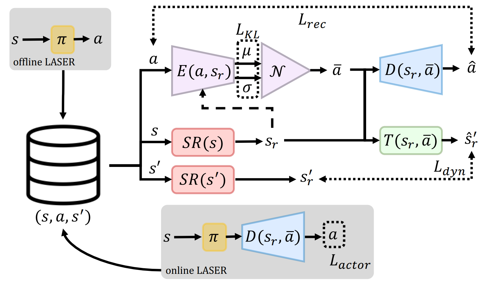
Looking for papers that implement this, I came across LASER, Learning a Latent Action Space for Efficient Reinforcement Learning.
The idea is to abstract away actions by dealing it in a latent space that might be easier to think about. The properties we want from the latent space is that
- Latent action should preserve important information of the original action, and be able to uniquely reconstruct it
- Latent action should make it easier to think about the state, and make the future more easily predictable
- Actions that results in similar outcome should be close together in latent space
- Sampling from a typical latent action distribution and acting them should naturally have higher rewards than sampling from atypical latent distribution
To achieve this, the collected state \(s\), action \(a\) and state transition \(s'\) from interacting with the environment are used to train an Encoder \(E(a, s)\) to encode actions into latent action \(\overline{a}\), Decoder \(D(\overline{a}, s)\) that decodes latent action into action as a variational autoencoder pair, and a latent state transition function \(\overline{T}(s, \overline{a})\) that predicts next state given previous state and latent action.
Then these are trained using
- Action Reconstruction loss: Squared error \(\| a - D(E(a, s), s) \|^2_2\) if continuous, or Cross entropy \(-a \log( D(E(a, s), s))\) if discrete
- Dynamics loss: Squared error \(\| s' - T(E(a, s), s) \|^2_2\)
- Regularization loss: KL divergence \(KL(N(μ, σ) \| N(0,I))\) where \(μ, σ \sim E(a, s)\)
- Policy loss: \(- Q_{policy}(E(a, s), s)\)
I’m still trying to figure out how to make this work with Q-learning still, I’m hoping this would solve the action order problem. This actually kind of works already, but it’s not working as well. This was mostly me throwing around ideas to see what sticks, and I would like to spend more time on this.
Results
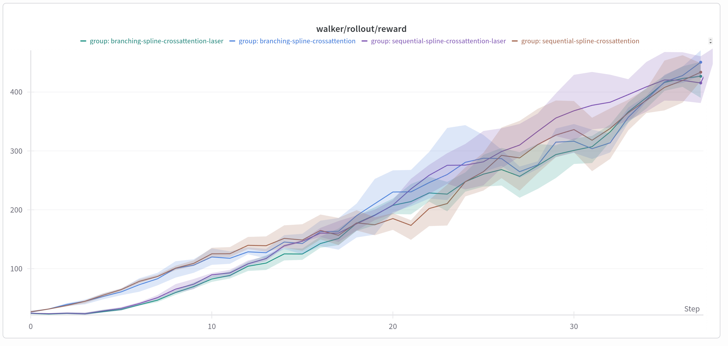
Results
Honestly I’m not sure what kind of conclusion I’m supposed to make out of the final results, since everything ended up performing pretty much the same as any other. Action Branching is actually pretty good, it turns out. It is also still faster to do, even if autoregressive sampling has many optimization points. For most environments, it’s probably fine to just do action branching, and see if my method is any better.
In some environments, Action Latents do much worse than not using it, while in other it’s about the same. Action Latent needs some warmup time where it only trains the action latent encoder, decoder and the dynamics model. During that time, the Q-Net doesn’t learn anything, but it seems to be getting better scores than random actions, which is kind of weird? My guess is that, even though it doesn’t know what actions are better or worse, doing things that lead to more interesting states generally have a higher reward, so maybe it can learn what actions achieve nothing and avoid doing them?
I think right now, I need more environments to test on. If every model reaches the same performance at the same time, it usually means you need a better test to see which are better.