Extending DQN to Continuous Action Spaces with Cubic Splines

One of the main things that turns people away from using Deep Q-Learning is its inability to handle continuous actions or multiple sub-actions. In Stable Baselines 3, they have a table of reinforcement learning algorithms and what kind of action spaces they each work in.
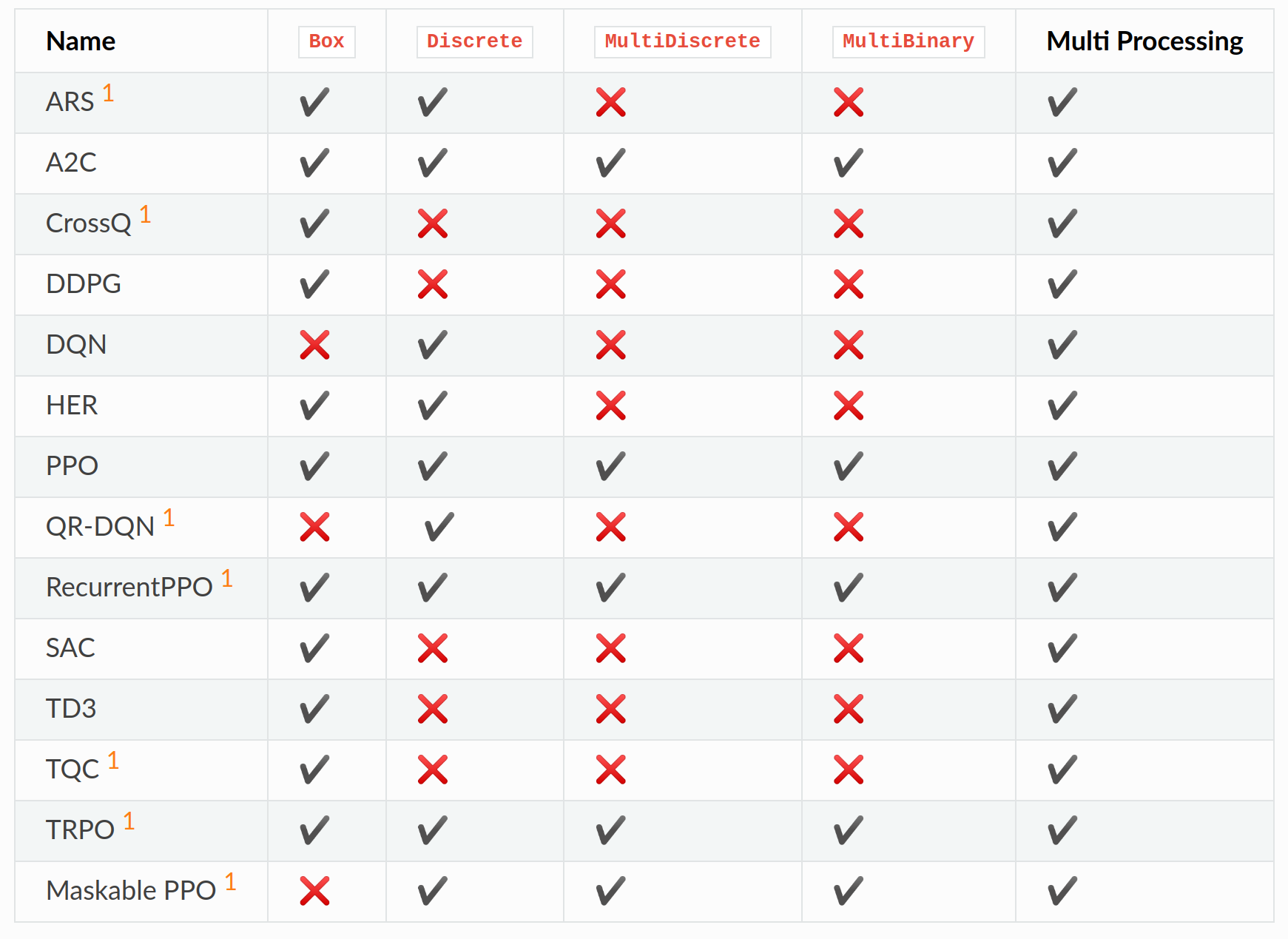
In their table, DQN only has a tick on the Discrete actions box. That is very limiting! It would be nice if there was an easy and cheap way of allowing DQN to work with continuous and multiple actions. But for now, let’s focus on how to make the first one work.
The Problem with Discrete-Only Actions
In games such fighting games, where an agent selects from a set of actions (move left, jump, shoot), a normal DQN works wonderfully. But what about games that need more precise control? Think about:
- A car adjusting its steering angle
- Twinstick shooter like Binding of Isaac
- A game like Minecraft where you need both discrete actions (moving with WASD keys, mining with click) and continuous control (moving the camera around)
Eventually I would have to build an agent that works with continuous control, but I knew DQN wouldn’t work out of the box. The standard approach-discretizing the action space into bins-technically works but produces jerky, unnatural movement. Imagine a car that can only turn its steering wheel in 10-degree increments instead of smoothly!
Most practitioners simply avoid DQN altogether for these tasks, moving to algorithms specifically designed for continuous control like DDPG or SAC. But I wondered: could we adapt DQN to handle continuous actions elegantly?
Why Can’t DQN Handle Continuous Actions?
To understand the problem, we need to revisit how Q-learning actually works.
In DQN, the Q-function represents the expected future reward when taking action a in state s, then following the policy afterward. This is written as $Q(s, a)$.
For an agent to act, it needs to find the action that maximizes this Q-function:
\[a^* = \arg\max_a Q(s, a)\]For discrete actions, this is straightforward. If you have 4 possible actions, you calculate a Q-value for each one and pick the highest. Done!
But what happens with continuous actions? If an action can be any value between, say, 0 and 1, we can’t simply enumerate all possibilities.

The Standard Solution: Discretization
The most common approach is to simply chop up (discretize) the continuous action space into a finite set of actions.
For example, if your action space is $[0, 1]$, you might use ${0, 0.1, 0.2, …, 0.9, 1.0}$ as your discrete approximation.

This works, but has significant drawbacks:
- Resolution problems: Too few points and your agent can’t make fine adjustments; too many and learning becomes inefficient
- No knowledge transfer: Learning that an action is good doesn’t tells the agent whether a similar action would also be good
- Curse of dimensionality: Discretizing multiple continuous actions leads to combinatorial explosion (more on this in next post!)
A Different Way of Looking at Q-Functions
Let’s think about what happens when we’re trying to select an action. Notice something important:
For a given state $s$, the argmax operation over actions doesn’t depend on the state anymore. We’ve essentially “locked in” our state and now just need to find the best action for that particular state.
This means, to make the argmax operation easier, we could curry the state into the Q-function $Q(s, a)$ to make a simpler function that only depends on the action $Q_s(a)$, and then take the maximum over the action:
\[Q_s(a) = Q(s, a) \text{ where } s \text{ is fixed}\]For discrete actions, $Q_s(a)$ is just a lookup table! Finding the maximum value in a table is trivial.
But for continuous actions, $Q_s(a)$ becomes a continuous function over the action space. Finding the maximum of an arbitrary continuous function is much harder.
What We Need in a Continuous Q-Function
If we want to use Q-learning with continuous actions, our representation of the Q-function needs to support several operations:
- Evaluation: We need to compute $Q(s, a)$ for any action $a$
- Maximization: We need to efficiently find the action $a$ that maximizes $Q(s, a)$
- Integration: For some advanced techniques like Dueling Networks, we need to compute the average Q-value across all actions
- Addition: We need to be able to add Q-functions together (useful for ensemble methods)

Many function approximators can handle evaluation, but maximization and integration are trickier. Neural networks, for instance, make evaluation easy but finding the global maximum is very difficult.
So what kind of mathematical construct could satisfy all these requirements?
Using Natural Cubic Splines
A cubic spline is a piecewise function made up of cubic polynomials that are smoothly connected at specific points called knots.
Cubic splines have several properties that make them perfect for our needs:
- They’re smooth and continuous
- They can approximate any continuous function (with enough knots)
- We can analytically find their maximums and compute their integrals
- They’re closed under addition (adding two cubic splines gives you another cubic spline)
How Cubic Splines Work
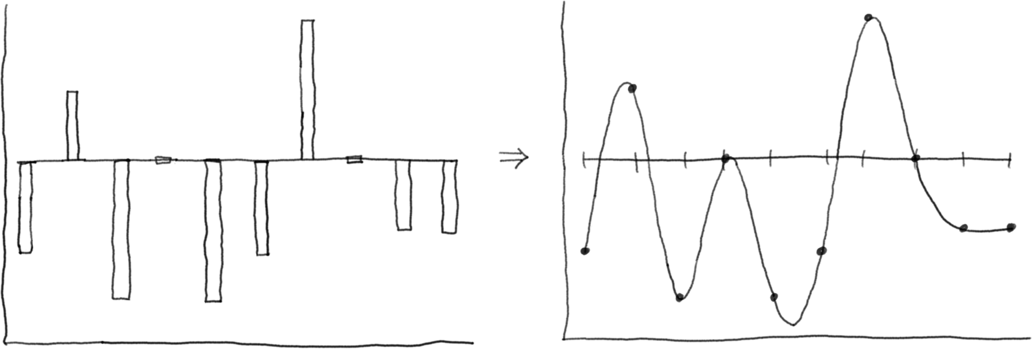
A cubic spline is defined by a set of control points (or knots) $(x_0, y_0), …, (x_n, y_n), (x_{n+1}, y_{n+1})$ where values $x$ are positions in our action space and values $y$ are our estimated Q-values at those actions.
Given these knots, the spline is
\[\begin{align}S(x) &= a_i t^3 + b_i t^2 + c_i t + d_i & \text{where} & & x_i \leq x \leq x_{i+1} & \text{,} & t = \frac{x-x_i}{x_{i+1} - x_i} \end{align}\]These polynomials are crafted to ensure that:
- The spline passes through all control points
- The first and second derivatives match at each interior control point
- Specific boundary conditions are met at the endpoints
I find that it’s much easier to handle if the internal coordinates of each polynomial goes from 0 to 1, and we translate when using them.
Check out WolframMathWorld for the cubic polynomial formula when the knots are equidistant, and the Addendum for non-equidistant knots.
Operations on Cubic Splines
Now let’s see how cubic splines handle all the operations we need:
1. Evaluation
To evaluate a cubic spline at a particular action value:
- Find which segment the action falls into
- Evaluate the cubic polynomial for that segment
2. Finding the Maximum
We can use the derivative tests to find all the potential points for each segment, and then find the maximum of those.
For each cubic polynomial segment:
- Calculate its derivative curve
- Find the roots of the derivative (1st derivative test)
- Evaluate the spline at these points and at the boundaries
- Take the maximum of all these values

Since we’re dealing with cubic polynomials, the derivative is quadratic, and finding roots of a quadratic equation is trivial using the quadratic formula
And we can even narrow down the points by half if we use the 2nd derivative test, halving the amount to search!
3. Computing the Mean
Taking the mean of the Q function over the action is needed in methods like Dueling Network and a few others.
The mean value of a function over the entire input could be computed by taking the integral and dividing by the input space size.
\[\mu = \int_{\min}^{\max} \frac{ S(x)}{\max - \min} dx\]For our cubic spline, we just need to integrate all the cubic polynomials and add them together, then multiply by the segment lengths they’re in.
If we made the internal coordinates go from 0 to 1, we don’t even need to integrate, it all simplifies to a single einsum expression
\[\frac{ \left[\frac{1}{4}, \frac{1}{3}, \frac{1}{2}, 1 \right]_i Coeff_{ij} \Delta x_j}{x_{n+1} - x_0}\]4. Adding Splines
Adding Q functions together is needed in some methods such as some extended Dueling Network or multi goal learning
Adding two cubic splines is straightforward:
- Combine all unique knot points
- For each segment in the combined domain, add the corresponding polynomial coefficients
Advantages of Spline
Using cubic splines to represent our Q-function gives us several advantages:
- Smooth approximation: Unlike discretization, splines provide a continuous representation with few points
- Knowledge transfer: Learning about the Q-value at one action informs us about nearby actions
- Analytical maximization: The optimal action can be found precisely and efficiently, without needing to evaluate the entire space
- Circular action spaces: Spline curves can have connected end points with continuous derivative, handling angles well
I am not aware of any easily usable environments with circular action spaces to experiment in yet, let me know if you do
Conclusion
DQN doesn’t have to be limited to discrete action spaces. By representing the Q-function as a cubic spline, we can enable DQN to work with continuous actions, without adding too much overhead.
Since splines are controlled by knots, it works with the exact input shape with what you would have used when doing discretized actions, making it pretty much a drop in replacement.
In the next post, I’ll show how to solve the other limitation with Q learning, handling mutliple subactions in a step without getting cursed by the dimensionality
Addendum
Prior Works
I have found some work on this, one is CAQL: CONTINUOUS ACTION Q-LEARNING where they make a tiny ReLU network and use Mixed Integer Programming, basically linear programming to find the maximum.
The method has limitations such as being slow, since each forward needs to solve an optimization problem, and only working when the action space is small, they only test on environments where the action space has been very limited.
I have found a work that uses spline curves for handling continuous action space, they call it Wire Fitting, it’s from 1993 and this is what the front page looks like
Experimental Results
Results
Here I put Weights and Bias plots of rewards for runs done with discretized action and spline action.
Environments are Reacher from MuJoCo and Walker and Finger environment from Deep Mind’s Control Suit
(click to enlarge)


Comparison of Walker performance between discretized action and spline action.


The discretized agent is doing a butt slide, this strategy seems to be a very stable way of moving and won’t fall over, but has a limit on how fast it can move.
The spline agent is running as fast as it can, losing balance but quickly able to stand up and fall down again. It seems like it’s prioritizing short term gain over long term gain.
Real time Q function graph of Reacher environment

Code Implementation
Spline Implementation
import torch
import einops

class SplineLayer(torch.nn.Module):
    def __init__(self, num_points, min = 0, max = 1):
        super().__init__()
        self.num_points = num_points
        self.min = min
        self.max = max

        self.register_buffer("inverse", self._precompute_inverse(), persistent = False)

    def _precompute_inverse(self):
        n = self.num_points

        diag = torch.ones(n) * 4
        diag[0] = diag[-1] = 2

        off_diag = torch.ones(n-1)
        A = torch.diag(diag) + torch.diag(off_diag, 1) + torch.diag(off_diag, -1)

        return torch.linalg.inv(A) * 3

    def _compute_coefficients(self, y):
        *batch_size, n = y.shape

        rhs = torch.zeros((*batch_size, n), device=y.device)
        rhs[..., 0] = (y[...,1]  - y[...,0])
        rhs[..., 1:-1] = (y[...,2:]- y[...,:-2])
        rhs[..., -1] = (y[..., -1]  - y[...,-2])

        D = torch.matmul(rhs, self.inverse)

        yi = y[..., :-1]
        yi1 = y[..., 1:]
        di = D[..., :-1]
        di1 = D[..., 1:]

        coeffs = torch.stack([(2*(yi-yi1)+di+di1),  (3 * (yi1-yi)-2*di-di1), di, yi], dim=-1)
        return coeffs

    def forward(self, points):
        coefficients = self._compute_coefficients(points)
        return Spline(points, coefficients, self.min,self.max)

class Spline:
    def __init__(self, points, coefficients, min = 0, max = 1):
        self.points = points
        self.coefficients = coefficients
        self.num_segments = coefficients.shape[-2]
        self.batch_shape = points.shape[:-1]
        self.max = max
        self.min = min

    def evaluate(self, t):
        if isinstance(t, (int, float)):
            t = torch.tensor([t], device=self.coefficients.device)
        else:
            t = t.to(self.coefficients.device)

        t = (t - self.min) / (self.max - self.min) * self.num_segments
        t = torch.clamp(t, 1e-6, self.num_segments-1e-6)

        seg = t.long()
        t = (t - seg.float())

        abcd = self.coefficients.gather(-2,seg[...,None].expand(*[-1]*len(seg.shape), 4))

        return ((abcd[...,0] * t + abcd[...,1]) * t + abcd[...,2]) * t + abcd[...,3]

    def maximum(self, dim = None, weight = 1):
        if dim is not None:
            a,b,c,d = (self.coefficients * weight).sum(dim).tensor_split((1,2,3), -1)
        else:
            a,b,c,d = self.coefficients.tensor_split((1,2,3), -1)
        aa = -3 * a

        dd = torch.sqrt(b.square() + aa * c)

        t = torch.clamp((b + dd) / aa, 0, 1)
        t[...,:-1,:] = t[...,:-1,:].nan_to_num(0.)
        t[...,-1,:] =t[...,-1,:].nan_to_num(1.)
        m = ((a * t + b) * t + c) * t + d

        p = m.max(-2)

        if dim is not None:
            indices = torch.ones(len(self.coefficients.shape), dtype = torch.int64)
            indices[-1] = 4
            indices[dim] = self.coefficients.shape[dim]
            abcd = self.coefficients.gather(-2,p.indices[...,None, None].expand(*indices))[..., 0, :]
            t = t[..., 0].gather(-1,p.indices)
            return ((abcd[...,0] * t + abcd[...,1]) * t + abcd[..., 2]) * t + abcd[..., 3], (t+p.indices)*(self.max - self.min)/self.num_segments + self.min
        else:
            return p.values, (t[..., 0].gather(-1, p.indices))*(self.max - self.min) + self.min

    def mean(self):
        return einops.einsum(self.coefficients, torch.tensor([1/4, 1/3, 1/2, 1],device=self.coefficients.device), '... s f, f -> ...') / self.num_segments
Non-equidistant Knot Case
Spline Formula
WolframMathWorld goes through the derivation of spline curve coefficients when the knots are equally spaced, but the case for arbitrary knots was hard to find for me.
The derivation is very similar but with few changes. First, we need to setup the problem.
Given a list of $ n $ knots $(x_i, y_i)$ where $ 0 = x_0 < x_1 < … < x_{i-1} < x_n = 1$
We want to define the spline curve $S(x)$ where $ 0 \leq x \leq 1 $.
We define
-
Segment lengths $ \Delta x_i = x_{i+1} - x_i $
-
$ S(x) = S_i(t) = a_i t^3 + b_i t^2 + c_i t + d_i $ where $ x_i \leq x \leq x_{i+1}$, $t = \frac{x-x_i}{\Delta x_i}$
Then
\[\begin{align} S_i(0) & = y_i & = d_i \\ S_i(1) & = y_{i+1} & = a_i + b_i + c_i + d_i \\ \end{align}\]When taking the derivative, we want it in respect to $x$ instead of $t$
\[\begin{align} S'_i(0) & = D_i & = \frac{c_i}{\Delta x_i} \\ S'_i(1) & = D_{i+1} & = \frac{(3a_i + 2b_i + c_i)}{\Delta x_i} \end{align}\]Solving for the coefficients gives
\[\begin{align} d_i & = y_i \\ c_i & = D_i \\ b_i & = 3(y_{i+1} - y_i) - (2 D_i + D_{i+1}) \Delta x_i\\ a_i & = 2(y_i - y_{i+1}) + (D_i + D_{i+1}) \Delta x_i \end{align}\]We now set the second derivative condition of natural spline
\[\begin{align} S''_0(0) = & 0 \\ S''_{i-1}(1) = & S''_i(0) \\ S''_n(1) = & 0 \end{align}\]Substituting the coefficients, we get
\[3y_1 - 3y_0 = \Delta x_0 D_1 +2 \Delta x_0 D_0\] \[\begin{multline} 3 \frac{\Delta x_{i-1}}{\Delta x_i} y_{i+1} + 3( \frac{\Delta x_i}{\Delta x_{i-1}} - \frac{\Delta x_{i-1}}{\Delta x_i}) y_i - 3 \frac{\Delta x_i}{\Delta x_{i-1}} y_{i-1} \\ = \Delta x_{i-1} D_{i+1} + 2 ( \Delta x_i + \Delta x_{i-1}) D_i + \Delta x_i D_{i-1} \end{multline}\] \[3y_n - 3y_{n-1} = \Delta x_n D_n +2 \Delta x_n D_{n-1}\]Which can be written as the matrix
\[\begin{split} \begin{bmatrix} 2 \Delta x_0 & \Delta x_0 & & & \cdots \\ \Delta x_1 & 2(\Delta x_0 + \Delta x_1) & \Delta x_0 & & \cdots \\ & \Delta x_2 & 2(\Delta x_1 + \Delta x_2) & \Delta x_1 & \cdots \\ \vdots & \vdots & \vdots & \vdots & \ddots & \\ & & \Delta x_{n-1} & 2(\Delta x_{n-2} + \Delta x_{n-1}) & \Delta x_{n-2} \\ & & & \Delta x_n & 2 \Delta x_n \end{bmatrix} \begin{bmatrix} D_0 \\ D_1 \\ D_2 \\ \vdots \\ D_{n-1} \\ D_n \end{bmatrix} \\ = 3 \begin{bmatrix} y_1 - y_0 \\ \frac{\Delta x_0}{\Delta x_1} y_2 + ( \frac{\Delta x_1}{\Delta x_0} - \frac{\Delta x_0}{\Delta x_1}) y_1 - \frac{\Delta x_1}{\Delta x_0} y_0 \\ \frac{\Delta x_1}{\Delta x_2} y_3 + ( \frac{\Delta x_2}{\Delta x_1} - \frac{\Delta x_1}{\Delta x_2}) y_2 - \frac{\Delta x_2}{\Delta x_1} y_1 \\ \vdots \\ \frac{\Delta x_{n-2}}{\Delta x_{n-1}} y_n + ( \frac{\Delta x_{n-1}}{\Delta x_{n-2}} - \frac{\Delta x_{n-2}}{\Delta x_{n-1}}) y_{n-1} - \frac{\Delta x_{n-1}}{\Delta x_{n-2}} y_{n-2} \\ y_n - y_{n-1} \end{bmatrix} \end{split}\]